※ This article is translated from Japanese version with some improvements on code.

Making simulation fast utilizing the power of GPU/TPU is a hot topic in the reinforcement learning community. LLM and RLHF things are getting ‘the thing’ in the community, though. Anyway, it is quite fun to speed up simulation. NVIDIA IsaacSym is quite solid, but if you want to speed up the entire RL pipeline, Jax-based libraries such as brax is useful.

You don’t know Jax? It’s just a NumPy-like library, but it can be compiled into a fast vectorized machine code that works really fast on GPU and TPU. It’s even fast on CPUs. I have written a blog post (Japanese only) before, but the current version of brax is farther improved. It allows you to choose a more accurate method, and it will be tightly integrated with MuJoCo XLA.

However, recently, I wanted a simple 2-D physics simulation, and tried brax. My impression was that not only brax is a complete overkill for my usecase, but also its API is quite difficult to set up a new environment. Loading MJCF is easy, but that was the only easy way to set up the stuff. I wanted to make my environment with some lines of Python code like game-physics engines such as pymunk. So, anyway, I tried to make my own.

Move things by semi-implicit Euler

Dealing with contacts is almost always the most diffucult in physics simulation. So, for now, let’s forget about that. Let’s just make things move. Let \(x, v\) denote the position and velocity, and \(\dot{x} = \frac{dx}{dt}, \dot{v} = \frac{dv}{dt}\) be their differentiations. From the second law, \(F(t) = m \frac{d^2 x}{dt^2}(t)\). Then, for a sufficiently small \(\Delta t\), the discrete time form of updating \(x\) and \(v\) is given:

\[ \begin{align*} \dot{x}_{t + 1} &= \dot{v}_t \Delta t \\ \dot{v}_{t + 1} &= \frac{F}{m} \Delta t . \end{align*} \]

This is unstable and rarely used. The simple trick I use is the Semi-implicit Euler, which just flips the order of update by:

\[ \begin{align*} \dot{v}_{t + 1} &= \frac{F}{m} \Delta t \\ \dot{x}_{t + 1} &= \dot{v}_{t + 1} \Delta t \end{align*} \] .

Now let’s start coding by defining structs, like Velocity. For shapes, let’s use Circle for now.

Code

from typing import Any, Protocol, Sequence

import chex
import jax
import jax.numpy as jnp

Self = Any


class PyTreeOps:
    def __add__(self, o: Any) -> Self:
        if o.__class__ is self.__class__:
            return jax.tree_map(lambda x, y: x + y, self, o)
        else:
            return jax.tree_map(lambda x: x + o, self)

    def __sub__(self, o: Any) -> Self:
        if o.__class__ is self.__class__:
            return jax.tree_map(lambda x, y: x - y, self, o)
        else:
            return jax.tree_map(lambda x: x - o, self)

    def __mul__(self, o: float | jax.Array) -> Self:
        return jax.tree_map(lambda x: x * o, self)

    def __neg__(self) -> Self:
        return jax.tree_map(lambda x: -x, self)

    def __truediv__(self, o: float | jax.Array) -> Self:
        return jax.tree_map(lambda x: x / o, self)

    def get_slice(
        self,
        index: int | Sequence[int] | Sequence[bool] | jax.Array,
    ) -> Self:
        return jax.tree_map(lambda x: x[index], self)

    def reshape(self, shape: Sequence[int]) -> Self:
        return jax.tree_map(lambda x: x.reshape(shape), self)

    def sum(self, axis: int | None = None) -> Self:
        return jax.tree_map(lambda x: jnp.sum(x, axis=axis), self)

    def tolist(self) -> list[Self]:
        leaves, treedef = jax.tree_util.tree_flatten(self)
        return [treedef.unflatten(leaf) for leaf in zip(*leaves)]

    def zeros_like(self) -> Any:
        return jax.tree_map(lambda x: jnp.zeros_like(x), self)

    @property
    def shape(self) -> Any:
        """For debugging"""
        return jax.tree_map(lambda x: x.shape, self)


TWO_PI = jnp.pi * 2


class _PositionLike(Protocol):
    angle: jax.Array  # Angular velocity (N,)
    xy: jax.Array  # (N, 2)

    def __init__(self, angle: jax.Array, xy: jax.Array) -> Self:
        ...

    def batch_size(self) -> int:
        return self.angle.shape[0]

    @classmethod
    def zeros(cls: type[Self], n: int) -> Self:
        return cls(angle=jnp.zeros((n,)), xy=jnp.zeros((n, 2)))


@chex.dataclass
class Velocity(_PositionLike, PyTreeOps):
    angle: jax.Array  # Angular velocity (N,)
    xy: jax.Array  # (N, 2)


@chex.dataclass
class Force(_PositionLike, PyTreeOps):
    angle: jax.Array  # Angular (torque) force (N,)
    xy: jax.Array  # (N, 2)


def _get_xy(xy: jax.Array) -> tuple[jax.Array, jax.Array]:
    x = jax.lax.slice_in_dim(xy, 0, 1, axis=-1)
    y = jax.lax.slice_in_dim(xy, 1, 2, axis=-1)
    return jax.lax.squeeze(x, (-1,)), jax.lax.squeeze(y, (-1,))


@chex.dataclass
class Position(_PositionLike, PyTreeOps):
    angle: jax.Array  # Angular velocity (N, 1)
    xy: jax.Array  # (N, 2)

    def rotate(self, xy: jax.Array) -> jax.Array:
        x, y = _get_xy(xy)
        s, c = jnp.sin(self.angle), jnp.cos(self.angle)
        rot_x = c * x - s * y
        rot_y = s * x + c * y
        return jnp.stack((rot_x, rot_y), axis=-1)

    def transform(self, xy: jax.Array) -> jax.Array:
        return self.rotate(xy) + self.xy

    def inv_rotate(self, xy: jax.Array) -> jax.Array:
        x, y = _get_xy(xy)
        s, c = jnp.sin(self.angle), jnp.cos(self.angle)
        rot_x = c * x + s * y
        rot_y = c * y - s * x
        return jnp.stack((rot_x, rot_y), axis=-1)

    def inv_transform(self, xy: jax.Array) -> jax.Array:
        return self.inv_rotate(xy - self.xy)


@chex.dataclass
class Shape(PyTreeOps):
    mass: jax.Array
    moment: jax.Array
    elasticity: jax.Array
    friction: jax.Array
    rgba: jax.Array

    def inv_mass(self) -> jax.Array:
        """To support static shape, set let inv_mass 0 if mass is infinite"""
        m = self.mass
        return jnp.where(jnp.isfinite(m), 1.0 / m, jnp.zeros_like(m))

    def inv_moment(self) -> jax.Array:
        """As inv_mass does, set inv_moment 0 if moment is infinite"""
        m = self.moment
        return jnp.where(jnp.isfinite(m), 1.0 / m, jnp.zeros_like(m))

    def to_shape(self) -> Self:
        return Shape(
            mass=self.mass,
            moment=self.moment,
            elasticity=self.elasticity,
            friction=self.friction,
            rgba=self.rgba,
        )


@chex.dataclass
class Circle(Shape):
    radius: jax.Array


@chex.dataclass
class State(PyTreeOps):
    p: Position
    v: Velocity
    f: Force
    is_active: jax.Array


@chex.dataclass
class Space:
    gravity: jax.Array
    circle: Circle
    dt: jax.Array | float = 0.1
    linear_damping: jax.Array | float = 0.95
    angular_damping: jax.Array | float = 0.95
    bias_factor: jax.Array | float = 0.2
    n_velocity_iter: int = 8
    n_position_iter: int = 2
    linear_slop: jax.Array | float = 0.005
    max_linear_correction: jax.Array | float = 0.2
    allowed_penetration: jax.Array | float = 0.005
    bounce_threshold: float = 1.0

Then let’s prepare some functions for drawing.

Code

from typing import Iterable

from matplotlib import pyplot as plt
from matplotlib.axes import Axes
from matplotlib.patches import Circle as CirclePatch
%matplotlib ipympl
plt.ioff()

def visualize_balls(ax: Axes, circles: Circle, positions: Iterable[Position]) -> None:
    pos = list(positions)
    circle_list = circles.tolist()
    for pi in pos:
        for pij, circle in zip(pi.tolist(), circle_list):
            circle_patch = CirclePatch(
                xy=pij.xy,
                radius=circle.radius,
                fill=False,
                color=circle.rgba.tolist(),
            )
            ax.add_patch(circle_patch)

Then, here is the Semi-implicit Euler.

Code

def update_velocity(space: Space, shape: Shape, state: State) -> State:
    # Expand (N, ) to (N, 1) because xy has a shape (N, 2)
    invm = jnp.expand_dims(shape.inv_mass(), axis=1)
    gravity = jnp.where(
        jnp.logical_and(invm > 0, jnp.expand_dims(state.is_active, axis=1)),
        space.gravity * jnp.ones_like(state.v.xy),
        jnp.zeros_like(state.v.xy),
    )
    v_xy = state.v.xy + (gravity + state.f.xy * invm) * space.dt
    v_ang = state.v.angle + state.f.angle * shape.inv_moment() * space.dt
    # Damping: dv/dt + vc = 0 -> v(t) = v0 * exp(-tc)
    # v(t + dt) = v0 * exp(-tc - dtc) = v0 * exp(-tc) * exp(-dtc) = v(t)exp(-dtc)
    # Thus, linear/angular damping factors are actually exp(-dtc)
    return state.replace(
        v=Velocity(angle=v_ang * space.angular_damping, xy=v_xy * space.linear_damping),
        f=state.f.zeros_like(),
    )


def update_position(space: Space, state: State) -> State:
    v_dt = state.v * space.dt
    xy = state.p.xy + v_dt.xy
    angle = (state.p.angle + v_dt.angle + TWO_PI) % TWO_PI
    return state.replace(p=Position(angle=angle, xy=xy))

Let’s just watch falling balls.

Code

circles = Circle(
    mass=jnp.ones(3),
    radius=jnp.ones(3),
    moment=jnp.ones(3) * 0.5,
    elasticity=jnp.ones(3),
    friction=jnp.ones(3),
    rgba=jnp.tile(jnp.array([0.2, 0.2, 0.2, 1.0]), (3, 1)),
)
space = Space(gravity=jnp.array([0.0, -9.8]), circle=circles)
p = Position(
    angle=jnp.array([-2, 0.1, 0.2]),
    xy=jnp.array([[-3, 4.0], [0.0, 2.0], [3.0, 3]]),
)
v = Velocity.zeros(3)
f = Force.zeros(3)
state = State(p=p, v=v, f=f, is_active=jnp.ones(3, dtype=bool))
positions = [state.p]
for i in range(20):
    state = update_velocity(space, circles, state)
    state = update_position(space, state)
    positions.append(state.p)
fig, ax = plt.subplots()
ax.set_aspect("equal", adjustable="box")
ax.set_xlim((-5, 5))
ax.set_ylim((-5, 5))
visualize_balls(ax, space.circle, positions)
fig

Looks OK?

Check contacts

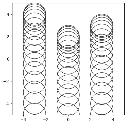
Next, let’s implement collision detection. It’s pretty easy because we have only circles now. We just need to store some information such as location and overwrap to resolve collisions later.

The other thing I need to care is vectorization. Say, this is a naive Python code to check contacts.

for i in range(N):
    for j in range(i + 1, N):
        check_contact(objects[i], objects[j])

It has \(O(N^2)\) loop! However, you might be smart enough to point out that each operation in this loop has no dependency, or the order of computation doesn’t matter. Here, jax.vmap is for you to vectorize those operations. Then, let’s unrole this loop by hand, make pairs, and then call check_contact. Like,

object_1, object_2 = make_pair(objects)
jax.vmap(check_contact)(object1, object2)

How to make pairs? There are various ways, what I found the simplest is triu_indices, which is a function that produces the indices of upper triangular matrix with some offsets.

Code

from typing import Any, Callable

Axis = Sequence[int] | int


def normalize(x: jax.Array, axis: Axis | None = None) -> tuple[jax.Array, jax.Array]:
    norm = jnp.linalg.norm(x, axis=axis)
    n = x / jnp.clip(norm, a_min=1e-6)
    return n, norm


@chex.dataclass
class Contact(PyTreeOps):
    pos: jax.Array
    normal: jax.Array
    penetration: jax.Array
    elasticity: jax.Array
    friction: jax.Array

    def contact_dim(self) -> int:
        return self.pos.shape[1]

@jax.vmap
def _circle_to_circle_impl(
    a: Circle,
    b: Circle,
    a_pos: Position,
    b_pos: Position,
    isactive: jax.Array,
) -> Contact:
    a2b_normal, dist = normalize(b_pos.xy - a_pos.xy)
    penetration = a.radius + b.radius - dist
    a_contact = a_pos.xy + a2b_normal * a.radius
    b_contact = b_pos.xy - a2b_normal * b.radius
    pos = (a_contact + b_contact) * 0.5
    # Filter penetration
    penetration = jnp.where(isactive, penetration, jnp.ones_like(penetration) * -1)
    return Contact(
        pos=pos,
        normal=a2b_normal,
        penetration=penetration,
        elasticity=(a.elasticity + b.elasticity) * 0.5,
        friction=(a.friction + b.friction) * 0.5,
    )


def check_circle_to_circle(
    space: Space,
    position: Position,
    is_active: jax.Array,
) -> tuple[Contact, Circle, Circle]:
    idx1, idx2 = jnp.triu_indices(is_active.shape[0], 1)
    circle1, circle2 = space.circle.get_slice(idx1), space.circle.get_slice(idx2)
    pos1, pos2 = position.get_slice(idx1), position.get_slice(idx2)
    is_active = jnp.logical_and(is_active[idx1], is_active[idx2])
    contacts = _circle_to_circle_impl(circle1, circle2, pos1, pos2, is_active)
    return contacts, circle1, circle2

Code

import seaborn as sns
from matplotlib.patches import Arrow

N = 5
palette = sns.color_palette("husl", N)


circles = Circle(
    mass=jnp.ones(N),
    radius=jnp.ones(N),
    moment=jnp.ones(N) * 0.5,
    elasticity=jnp.ones(N) * 0.5,
    friction=jnp.ones(N) * 0.2,
    rgba=jnp.array([p + (1.0,) for p in palette]),
)
space = Space(gravity=jnp.array([0.0, -9.8]), circle=circles)
p = Position(
    angle=jnp.zeros(N),
    xy=jnp.array([[-3, 4.0], [0.0, 2.0], [5.0, 3], [-3, 1], [2, 0]]),
)
v_xy = jnp.concatenate((jnp.zeros((N - 2, 2)), jnp.array([[0, 10.0], [-2.0, 8.0]])))
v = Velocity(angle=jnp.zeros(N), xy=v_xy)
f = Force(angle=jnp.zeros(N), xy=jnp.zeros((N, 2)))
state = State(p=p, v=v, f=f, is_active=jnp.ones(N, dtype=bool))
positions = [state.p]
contact_list = []
for i in range(10):
    state = update_velocity(space, circles, state)
    state = update_position(space, state)
    positions.append(state.p)
    contacts, _, _ = check_circle_to_circle(space, state.p, state.is_active)
    total_index = 0
    for j in range(N):
        for k in range(j + 1, N):
            if contacts.penetration[total_index] > 0:
                contact_list.append(contacts.get_slice(total_index))
            total_index += 1
fig, ax = plt.subplots()
ax.set_aspect("equal", adjustable="box")
ax.set_xlim((-5, 5))
ax.set_ylim((-5, 5))
visualize_balls(ax, space.circle, positions)
for contact in contact_list:
    arrow = Arrow(*contact.pos, *contact.normal, width=0.2, color="r")
    ax.add_patch(arrow)
fig

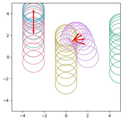
Objects are overlapping since I haven’t implemented resolving collision, but the dected collision looks correct.

What to do after collision detection

I’m not quite familiar with physics actually, but in the real world, collisions are automatically resolved by each small molecule. But in the game physics engine, we want to get results faster by enforcing physically acurate constraints, such as:

Speed changes by collision
No overlap between objects

So, I’m just solving these constraints. There are many ways to solve these, but here, I employ a common approach called Sequential Impulse, which is used in a famous physics engines including Chipmunk and Box2D. Other approaches includes recently trending position-based dynamics, but sequatinal impulse caught my eyes because of its simplicity.

Anyway, let me explain how sequential impulse method resolves collision. First, let’s assume a collision model in which collision produces impulse, and let the generated impulse be \(\mathbf{p}\). I don’t use angular velocity here for simplicity. Let the velocity and mass of object 1 be \(\mathbf{v}_1\) and \(m_1\), and the velocity and mass of object 2 be \(\mathbf{v}_2\) and \(m_2\), respectively, then the velocity after the impulse occurs is

\[ \begin{align*} \mathbf{v}_1 = \mathbf{v}_1^{\mathrm{old}} - \mathbf{p} / m_1 \\ \mathbf{v}_2 = \mathbf{v}_2^{\mathrm{old}} + \mathbf{p} / m_2 \end{align*} \]

Here, because the direction of \(\mathbf{p}\) is the normal vector of collision \(\mathbf{n}\), we can write that \(\mathbf{p} = p\mathbf{n}\). Hence, we just need to compute \(p\). Let the relative velocity at the collision point be \(\Delta \mathbf{v} = \mathbf{v}_2 - \mathbf{v}_1\). Here combining the avove two equalities with \(\Delta \mathbf{v} \cdot n = 0\), \(p = \frac{-\Delta \mathbf{v}^{\mathrm{old}}\cdot \mathbf{n}}{\frac{1}{m_1} + \frac{1}{m_2}}\). Angle makes this a bit more complicated, but the core equation is just like this.

こうして計算したインパルスを全ての衝突に対して適用し、インパルスが小さくなるまで繰り返します。しかし、この手法は物体のめりこみを考慮していないので、これだけだと物体がめりこんだままになってしまうことがあります。めり込みを減らすための手法はいくつかありますが、主に

どのくらいめり込んでいるかに応じてバイアス速度\(v_\mathrm{bias} = \frac{\beta}{\Delta t}\max(0, \delta - \delta_\mathrm{slop})\)(\(\delta\)はめりこみの長さ、\(\delta_\mathrm{slop}\)は許容されるめりこみの長さ)を加え\(p = \frac{-\Delta \mathbf{v}^{\mathrm{old}}\cdot \mathbf{n} + v_\mathrm{bias}}{\frac{1}{m_1} + \frac{1}{m_2}}\)とする (Baumegarte)
速度を更新した後にもう一回Positionに関する制約を解いて擬似的な速度を加える (Nonlinear Gauss Seidel, NGS)

という2種類の手法があります。先程紹介したBox2Dの資料やChipmunk2Dでは1が、現在のBox2Dでは2が使われています。詳しくはBox2D 3.0のコメントを参照してください。今回は若干高速な1の手法を実装しようかと思ったのですが、この方法だと2つの物体が同じ方向に進んでいる時はめりこみを解消できないので、結局2の手法を実装しました。具体的にソルバの実装としては、

衝突により発生するインパルスに関する制約を解く
弾性により発生するインパルスを加える
位置に関する制約を解く

という3つのステップに分けて実装すればいいです。

また、さっき並列化のため手動で全ペアに対するループをアンロールしましたが、Sequential Impulseの実装でもこれが使えます。ただし、インパルスを加えた後の速度の更新は、v_update[i][j]にi番目の物体とj番目の物体の衝突により生じるi番目の物体の速度変化が入っているとして、

for i in range(N):
    for j in range(i + 1, N):
        obj[i].velocity += v_update[i][j]
        obj[j].velocity += v_update[j][i]

のように各衝突により生じた速度変化を物体にフィードバックする必要があります。これもいちいちループで書くと遅くなってしまうのですが、さっきのgenerate_self_pairsで\(0, 1, 2, ..., N - 1\)のペアを生成しておいてインデックスにするとループなしで書けます。細かく言うと、generate_self_pairsではループが使われているのですが、jax.jitでコンパイルした時に計算結果がキャッシュされるはずなので気にしなくてもいいです。

というわけで実装してみましょう。実装は基本的にBox2d-Liteと開発中の最新版であるBox2D 3.0を参考にしました。また、Box2D作者のErin Catto氏による講演の内容をTypescriptで実装したリポジトリがあったのでこれも参考にしました。

Code

import functools


@chex.dataclass
class ContactHelper:
    tangent: jax.Array
    mass_normal: jax.Array
    mass_tangent: jax.Array
    v_bias: jax.Array
    bounce: jax.Array
    r1: jax.Array
    r2: jax.Array
    inv_mass1: jax.Array
    inv_mass2: jax.Array
    inv_moment1: jax.Array
    inv_moment2: jax.Array
    local_anchor1: jax.Array
    local_anchor2: jax.Array
    allow_bounce: jax.Array


@chex.dataclass
class VelocitySolver:
    v1: Velocity
    v2: Velocity
    pn: jax.Array
    pt: jax.Array
    contact: jax.Array

    def update(self, new_contact: jax.Array) -> Self:
        continuing_contact = jnp.logical_and(self.contact, new_contact)
        pn = jnp.where(continuing_contact, self.pn, jnp.zeros_like(self.pn))
        pt = jnp.where(continuing_contact, self.pt, jnp.zeros_like(self.pt))
        return self.replace(pn=pn, pt=pt, contact=new_contact)


def init_solver(n: int) -> VelocitySolver:
    return VelocitySolver(
        v1=Velocity.zeros(n),
        v2=Velocity.zeros(n),
        pn=jnp.zeros(n),
        pt=jnp.zeros(n),
        contact=jnp.zeros(n, dtype=bool),
    )


def _pv_gather(
    p1: _PositionLike,
    p2: _PositionLike,
    orig: _PositionLike,
) -> _PositionLike:
    indices = jnp.arange(len(orig.angle))
    outer, inner = generate_self_pairs(indices)
    p1_xy = jnp.zeros_like(orig.xy).at[outer].add(p1.xy)
    p1_angle = jnp.zeros_like(orig.angle).at[outer].add(p1.angle)
    p2_xy = jnp.zeros_like(orig.xy).at[inner].add(p2.xy)
    p2_angle = jnp.zeros_like(orig.angle).at[inner].add(p2.angle)
    return p1.__class__(xy=p1_xy + p2_xy, angle=p1_angle + p2_angle)


def _vmap_dot(xy1: jax.Array, xy2: jax.Array) -> jax.Array:
    """Dot product between nested vectors"""
    chex.assert_equal_shape((xy1, xy2))
    orig_shape = xy1.shape
    a = xy1.reshape(-1, orig_shape[-1])
    b = xy2.reshape(-1, orig_shape[-1])
    return jax.vmap(jnp.dot, in_axes=(0, 0))(a, b).reshape(*orig_shape[:-1])


def _sv_cross(s: jax.Array, v: jax.Array) -> jax.Array:
    """Cross product with scalar and vector"""
    x, y = _get_xy(v)
    return jnp.stack((y * -s, x * s), axis=-1)


def _dv2from1(v1: Velocity, r1: jax.Array, v2: Velocity, r2: jax.Array) -> jax.Array:
    """Compute relative veclotiy from v2/r2 to v1/r1"""
    rel_v1 = v1.xy + _sv_cross(v1.angle, r1)
    rel_v2 = v2.xy + _sv_cross(v2.angle, r2)
    return rel_v2 - rel_v1


def _effective_mass(
    inv_mass: jax.Array,
    inv_moment: jax.Array,
    r: jax.Array,
    n: jax.Array,
) -> jax.Array:
    rn2 = jnp.cross(r, n) ** 2
    return inv_mass + inv_moment * rn2


def init_contact_helper(
    space: Space,
    contact: Contact,
    a: Shape,
    b: Shape,
    p1: Position,
    p2: Position,
    v1: Velocity,
    v2: Velocity,
) -> ContactHelper:
    r1 = contact.pos - p1.xy
    r2 = contact.pos - p2.xy

    inv_mass1, inv_mass2 = a.inv_mass(), b.inv_mass()
    inv_moment1, inv_moment2 = a.inv_moment(), b.inv_moment()
    kn1 = _effective_mass(inv_mass1, inv_moment1, r1, contact.normal)
    kn2 = _effective_mass(inv_mass2, inv_moment2, r2, contact.normal)
    nx, ny = _get_xy(contact.normal)
    tangent = jnp.stack((-ny, nx), axis=-1)
    kt1 = _effective_mass(inv_mass1, inv_moment1, r1, tangent)
    kt2 = _effective_mass(inv_mass2, inv_moment2, r2, tangent)
    clipped_p = jnp.clip(space.allowed_penetration - contact.penetration, a_max=0.0)
    v_bias = -space.bias_factor / space.dt * clipped_p
    # k_normal, k_tangent, and v_bias should have (N(N-1)/2, N_contacts) shape
    chex.assert_equal_shape((contact.friction, kn1, kn2, kt1, kt2, v_bias))
    # Compute elasiticity * relative_vel
    dv = _dv2from1(v1, r1, v2, r2)
    vn = _vmap_dot(dv, contact.normal)
    return ContactHelper(
        tangent=tangent,
        mass_normal=1 / (kn1 + kn2),
        mass_tangent=1 / (kt1 + kt2),
        v_bias=v_bias,
        bounce=vn * contact.elasticity,
        r1=r1,
        r2=r2,
        inv_mass1=inv_mass1,
        inv_mass2=inv_mass2,
        inv_moment1=inv_moment1,
        inv_moment2=inv_moment2,
        local_anchor1=p1.inv_rotate(r1),
        local_anchor2=p2.inv_rotate(r2),
        allow_bounce=vn <= -space.bounce_threshold,
    )


@jax.vmap
def apply_initial_impulse(
    contact: Contact,
    helper: ContactHelper,
    solver: VelocitySolver,
) -> VelocitySolver:
    """Warm starting by applying initial impulse"""
    p = helper.tangent * solver.pt + contact.normal * solver.pn
    v1 = solver.v1 - Velocity(
        angle=helper.inv_moment1 * jnp.cross(helper.r1, p),
        xy=p * helper.inv_mass1,
    )
    v2 = solver.v2 + Velocity(
        angle=helper.inv_moment2 * jnp.cross(helper.r2, p),
        xy=p * helper.inv_mass2,
    )
    return solver.replace(v1=v1, v2=v2)


@jax.vmap
def apply_velocity_normal(
    contact: Contact,
    helper: ContactHelper,
    solver: VelocitySolver,
) -> VelocitySolver:
    """
    Apply velocity constraints to the solver.
    Suppose that each shape has (N_contact, 1) or (N_contact, 2).
    """
    # Relative veclocity (from shape2 to shape1)
    dv = _dv2from1(solver.v1, helper.r1, solver.v2, helper.r2)
    vt = jnp.dot(dv, helper.tangent)
    dpt = -helper.mass_tangent * vt
    # Clamp friction impulse
    max_pt = contact.friction * solver.pn
    pt = jnp.clip(solver.pt + dpt, a_min=-max_pt, a_max=max_pt)
    dpt_clamped = helper.tangent * (pt - solver.pt)
    # Velocity update by contact tangent
    dvt1 = Velocity(
        angle=-helper.inv_moment1 * jnp.cross(helper.r1, dpt_clamped),
        xy=-dpt_clamped * helper.inv_mass1,
    )
    dvt2 = Velocity(
        angle=helper.inv_moment2 * jnp.cross(helper.r2, dpt_clamped),
        xy=dpt_clamped * helper.inv_mass2,
    )
    # Compute Relative velocity again
    dv = _dv2from1(solver.v1 + dvt1, helper.r1, solver.v2 + dvt2, helper.r2)
    vn = _vmap_dot(dv, contact.normal)
    dpn = helper.mass_normal * (-vn + helper.v_bias)
    # Accumulate and clamp impulse
    pn = jnp.clip(solver.pn + dpn, a_min=0.0)
    dpn_clamped = contact.normal * (pn - solver.pn)
    # Velocity update by contact normal
    dvn1 = Velocity(
        angle=-helper.inv_moment1 * jnp.cross(helper.r1, dpn_clamped),
        xy=-dpn_clamped * helper.inv_mass1,
    )
    dvn2 = Velocity(
        angle=helper.inv_moment2 * jnp.cross(helper.r2, dpn_clamped),
        xy=dpn_clamped * helper.inv_mass2,
    )
    # Filter dv
    dv1, dv2 = jax.tree_map(
        lambda x: jnp.where(solver.contact, x, jnp.zeros_like(x)),
        (dvn1 + dvt1, dvn2 + dvt2),
    )
    # Summing up dv per each contact pair
    return VelocitySolver(
        v1=dv1,
        v2=dv2,
        pn=pn,
        pt=pt,
        contact=solver.contact,
    )


@jax.vmap
def apply_bounce(
    contact: Contact,
    helper: ContactHelper,
    solver: VelocitySolver,
) -> tuple[Velocity, Velocity]:
    """
    Apply bounce (resititution).
    Suppose that each shape has (N_contact, 1) or (N_contact, 2).
    """
    # Relative veclocity (from shape2 to shape1)
    dv = _dv2from1(solver.v1, helper.r1, solver.v2, helper.r2)
    vn = jnp.dot(dv, contact.normal)
    pn = -helper.mass_normal * (vn + helper.bounce)
    dpn = contact.normal * pn
    # Velocity update by contact normal
    dv1 = Velocity(
        angle=-helper.inv_moment1 * jnp.cross(helper.r1, dpn),
        xy=-dpn * helper.inv_mass1,
    )
    dv2 = Velocity(
        angle=helper.inv_moment2 * jnp.cross(helper.r2, dpn),
        xy=dpn * helper.inv_mass2,
    )
    # Filter dv
    allow_bounce = jnp.logical_and(solver.contact, helper.allow_bounce)
    return jax.tree_map(
        lambda x: jnp.where(allow_bounce, x, jnp.zeros_like(x)),
        (dv1, dv2),
    )


@chex.dataclass
class PositionSolver:
    p1: Position
    p2: Position
    contact: jax.Array
    min_separation: jax.Array


@functools.partial(jax.vmap, in_axes=(None, None, None, 0, 0, 0))
def correct_position(
    bias_factor: float | jax.Array,
    linear_slop: float | jax.Array,
    max_linear_correction: float | jax.Array,
    contact: Contact,
    helper: ContactHelper,
    solver: PositionSolver,
) -> PositionSolver:
    """
    Correct positions to remove penetration.
    Suppose that each shape in contact and helper has (N_contact, 1) or (N_contact, 2).
    p1 and p2 should have xy: (1, 2) angle (1, 1) shape
    """
    # (N_contact, 2)
    r1 = solver.p1.rotate(helper.local_anchor1)
    r2 = solver.p2.rotate(helper.local_anchor2)
    ga2_ga1 = r2 - r1 + solver.p2.xy - solver.p1.xy
    separation = jnp.dot(ga2_ga1, contact.normal) - contact.penetration
    c = jnp.clip(
        bias_factor * (separation + linear_slop),
        a_min=-max_linear_correction,
        a_max=0.0,
    )
    kn1 = _effective_mass(helper.inv_mass1, helper.inv_moment1, r1, contact.normal)
    kn2 = _effective_mass(helper.inv_mass2, helper.inv_moment2, r2, contact.normal)
    k_normal = kn1 + kn2
    impulse = jnp.where(k_normal > 0.0, -c / k_normal, jnp.zeros_like(c))
    pn = impulse * contact.normal
    p1 = Position(
        angle=-helper.inv_moment1 * jnp.cross(r1, pn),
        xy=-pn * helper.inv_mass1,
    )
    p2 = Position(
        angle=helper.inv_moment2 * jnp.cross(r2, pn),
        xy=pn * helper.inv_mass2,
    )
    min_sep = jnp.fmin(solver.min_separation, separation)
    # Filter separation
    p1, p2 = jax.tree_map(
        lambda x: jnp.where(solver.contact, x, jnp.zeros_like(x)),
        (p1, p2),
    )
    return solver.replace(p1=p1, p2=p2, min_separation=min_sep)


def fake_fori_loop(start, end, step, initial):
    """For debugging. Just replace jax.lax.fori_loop with this."""
    state = initial
    for i in range(start, end):
        state = step(i, state)
    return state


def apply_seq_impulses(
    space: Space,
    solver: VelocitySolver,
    p: Position,
    v: Velocity,
    contact: Contact,
    a: Shape,
    b: Shape,
) -> tuple[Velocity, Position, VelocitySolver]:
    """Resolve collisions by Sequential Impulse method"""
    p1, p2 = tree_map2(generate_self_pairs, p)
    v1, v2 = tree_map2(generate_self_pairs, v)
    helper = init_contact_helper(space, contact, a, b, p1, p2, v1, v2)
    solver = apply_initial_impulse(
        contact,
        helper,
        solver.replace(v1=v1, v2=v2),
    )

    def vstep(
        _n_iter: int,
        vs: tuple[Velocity, VelocitySolver],
    ) -> tuple[Velocity, VelocitySolver]:
        v_i, solver_i = vs
        solver_i1 = apply_velocity_normal(contact, helper, solver_i)
        v_i1 = _pv_gather(solver_i1.v1, solver_i1.v2, v_i) + v_i
        v1, v2 = tree_map2(generate_self_pairs, v_i1)
        return v_i1, solver_i1.replace(v1=v1, v2=v2)

    v, solver = jax.lax.fori_loop(0, space.n_velocity_iter, vstep, (v, solver))
    rest_v1, rest_v2 = apply_bounce(contact, helper, solver)
    v = _pv_gather(rest_v1, rest_v2, v) + v

    def pstep(
        _n_iter: int,
        ps: tuple[Position, PositionSolver],
    ) -> tuple[Position, PositionSolver]:
        p_i, solver_i = ps
        solver_i1 = correct_position(
            space.bias_factor,
            space.linear_slop,
            space.max_linear_correction,
            contact,
            helper,
            solver_i,
        )
        p_i1 = _pv_gather(solver_i1.p1, solver_i1.p2, p_i) + p_i
        p1, p2 = tree_map2(generate_self_pairs, p_i1)
        return p_i1, solver_i1.replace(p1=p1, p2=p2)

    pos_solver = PositionSolver(
        p1=p1,
        p2=p2,
        contact=solver.contact,
        min_separation=jnp.zeros_like(p1.angle),
    )
    p, pos_solver = jax.lax.fori_loop(0, space.n_position_iter, pstep, (p, pos_solver))
    return v, p, solver

なかなか複雑になりましたが、実装できました。衝突させてみましょう。

Code

from celluloid import Camera
from IPython.display import HTML


def animate_balls(
    fig,
    ax: Axes,
    circles: Circle,
    positions: Iterable[Position],
) -> HTML:
    pos = list(positions)
    camera = Camera(fig)
    circle_list = circles.tolist()
    for pi in pos:
        for pij, circle in zip(pi.tolist(), circle_list):
            circle_patch = CirclePatch(
                xy=pij.xy,
                radius=circle.radius,
                fill=False,
                color=circle.rgba.tolist(),
            )
            ax.add_patch(circle_patch)
        camera.snap()
    return HTML(camera.animate().to_jshtml())

Code

space = Space(gravity=jnp.array([0.0, -9.8]), dt=0.04, bias_factor=0.2, circle=circles)
state = State(p=p, v=v, f=f, is_active=jnp.ones(N, dtype=bool))
positions = [state.p]
solver = init_solver(N * (N - 1) // 2)


@jax.jit
def step(state: State, solver: VelocitySolver) -> tuple[State, VelocitySolver]:
    state = update_velocity(space, space.circle, state)
    contacts, c1, c2 = check_circle_to_circle(space, state.p, state.is_active)
    v, p, solver = apply_seq_impulses(
        space,
        solver.update(contacts.penetration >= 0),
        state.p,
        state.v,
        contacts,
        c1,
        c2,
    )
    return update_position(space, state.replace(v=v, p=p)), solver


for i in range(30):
    state, solver = step(state, solver)
    positions.append(state.p)
fig, ax = plt.subplots()
ax.set_aspect("equal", adjustable="box")
ax.set_xlim((-10, 10))
ax.set_ylim((-10, 10))
animate_balls(fig, ax, space.circle, positions)

最初の衝突で若干のめりこみが発生していますが、一応大丈夫そうですね。

線分

円同士の衝突が実装できたところで、次は凸多角形の実装…と言いたいところですが、それは後回しにして、ゲームには欠かせない「線分」を実装してみます。現実世界にはそんなもの存在しないのですが、ゲームやシミュレーションの世界では、どうしても地面や柵といった境界を表現する必要が生じてきます。こういったものを例えば「めちゃくちゃ重い長方形」として表現することもできますが、シミュレーションを組むユーザー側からするといちいち長方形の大きさだったりを定義するのは面倒なので、「無限の質量を持つ線」として扱えたほうが楽ですよね。というわけで線分を実装してみます。線分の衝突判定は薬のカプセル💊のように両端が丸くなっているやつ(Box2Dだとカプセルと呼ばれているのでカプセルと呼びます)と実装がほぼ同じなので、カプセルも一緒に実装してしまいます。ただカプセル同士の衝突は面倒なので、とりあえず円とカプセルだけ実装しましょう。新しい図形を加えたので、Spaceも作り直す必要があります。とりあえずdataclassに全シェイプをつっこんでおいて、各シェイプの組み合わせごとに衝突判定を行い、衝突解決のときはjnp.concatenateで全部くっつけてからvmapで一度にやるという実装方針にしました。さっきのペアに対するループをアンロールするところは、インデックスのペアを持っておいて適当なオフセットを足しておけばそのまま使えます。

Code

from matplotlib.patches import Rectangle

@chex.dataclass
class Capsule(Shape):
    length: jax.Array
    radius: jax.Array


@chex.dataclass
class Segment(Shape):
    length: jax.Array

    def to_capsule(self) -> Capsule:
        return Capsule(
            mass=self.mass,
            moment=self.moment,
            elasticity=self.elasticity,
            friction=self.friction,
            rgba=self.rgba,
            length=self.length,
            radius=jnp.zeros_like(self.length),
        )


def _length_to_points(length: jax.Array) -> tuple[jax.Array, jax.Array]:
    a = jnp.stack((length * -0.5, length * 0.0), axis=-1)
    b = jnp.stack((length * 0.5, length * 0.0), axis=-1)
    return a, b


@jax.vmap
def _capsule_to_circle_impl(
    a: Capsule,
    b: Circle,
    a_pos: Position,
    b_pos: Position,
    isactive: jax.Array,
) -> Contact:
    # Move b_pos to capsule's coordinates
    pb = a_pos.inv_transform(b_pos.xy)
    p1, p2 = _length_to_points(a.length)
    edge = p2 - p1
    s1 = jnp.dot(pb - p1, edge)
    s2 = jnp.dot(p2 - pb, edge)
    in_segment = jnp.logical_and(s1 >= 0.0, s2 >= 0.0)
    ee = jnp.sum(jnp.square(edge), axis=-1, keepdims=True)
    # Closest point
    # s1 < 0: pb is left to the capsule
    # s2 < 0: pb is right to the capsule
    # else: pb is in between capsule
    pa = jax.lax.select(
        in_segment,
        p1 + edge * s1 / ee,
        jax.lax.select(s1 < 0.0, p1, p2),
    )
    a2b_normal, dist = normalize(pb - pa)
    penetration = a.radius + b.radius - dist
    a_contact = pa + a2b_normal * a.radius
    b_contact = pb - a2b_normal * b.radius
    pos = a_pos.transform((a_contact + b_contact) * 0.5)
    xy_zeros = jnp.zeros_like(b_pos.xy)
    a2b_normal_rotated = a_pos.replace(xy=xy_zeros).transform(a2b_normal)
    # Filter penetration
    penetration = jnp.where(isactive, penetration, jnp.ones_like(penetration) * -1)
    return Contact(
        pos=pos,
        normal=a2b_normal_rotated,
        penetration=penetration,
        elasticity=(a.elasticity + b.elasticity) * 0.5,
        friction=(a.friction + b.friction) * 0.5,
    )


@chex.dataclass
class ShapeDict:
    circle: Circle | None = None
    segment: Segment | None = None
    capsule: Capsule | None = None
    
    def concat(self) -> Shape:
        shapes = [s.to_shape() for s in self.values() if s is not None]
        return jax.tree_map(lambda *args: jnp.concatenate(args, axis=0), *shapes)


@chex.dataclass
class StateDict:
    circle: State | None = None
    segment: State | None = None
    capsule: State | None = None

    def concat(self) -> None:
        states = [s for s in self.values() if s is not None]
        return jax.tree_map(lambda *args: jnp.concatenate(args, axis=0), *states)

    def offset(self, key: str) -> int:
        total = 0
        for k, state in self.items():
            if k == key:
                return total
            if state is not None:
                total += state.p.batch_size()
        raise RuntimeError("Unreachable")
        
    def _get(self, name: str, state: State) -> State | None:
        if self[name] is None:
            return None
        else:
            start = self.offset(name)
            end = start + self[name].p.batch_size()
            return state.get_slice(jnp.arange(start, end))
        
    def update(self, statec: State) -> Self:
        circle = self._get("circle", statec)
        segment = self._get("segment", statec)
        capsule = self._get("capsule", statec)
        return self.__class__(circle=circle, segment=segment, capsule=capsule)


ContactFn = Callable[[StateDict], tuple[Contact, Shape, Shape]]


def _pair_outer(x: jax.Array, reps: int) -> jax.Array:
    return jnp.repeat(x, reps, axis=0, total_repeat_length=x.shape[0] * reps)


def _pair_inner(x: jax.Array, reps: int) -> jax.Array:
    return jnp.tile(x, (reps,) + (1,) * (x.ndim - 1))


def generate_pairs(x: jax.Array, y: jax.Array) -> tuple[jax.Array, jax.Array]:
    """Returns two arrays that iterate over all combination of elements in x and y"""
    xlen, ylen = x.shape[0], y.shape[0]
    return _pair_outer(x, ylen), _pair_inner(y, xlen)


def _circle_to_circle(
    shaped: ShapeDict,
    stated: StateDict,
) -> tuple[Contact, Circle, Circle]:
    circle1, circle2 = tree_map2(generate_self_pairs, shaped.circle)
    pos1, pos2 = tree_map2(generate_self_pairs, stated.circle.p)
    is_active = jnp.logical_and(*generate_self_pairs(stated.circle.is_active))
    contacts = _circle_to_circle_impl(
        circle1,
        circle2,
        pos1,
        pos2,
        is_active,
    )
    return contacts, circle1, circle2


def _capsule_to_circle(
    shaped: ShapeDict,
    stated: StateDict,
) -> tuple[Contact, Capsule, Circle]:
    capsule = jax.tree_map(
        functools.partial(_pair_outer, reps=shaped.circle.mass.shape[0]),
        shaped.capsule,
    )
    circle = jax.tree_map(
        functools.partial(_pair_inner, reps=shaped.capsule.mass.shape[0]),
        shaped.circle,
    )
    pos1, pos2 = tree_map2(generate_pairs, stated.capsule.p, stated.circle.p)
    is_active = jnp.logical_and(
        *generate_pairs(stated.capsule.is_active, stated.circle.is_active)
    )
    contacts = _capsule_to_circle_impl(
        capsule,
        circle,
        pos1,
        pos2,
        is_active,
    )
    return contacts, capsule, circle


def _segment_to_circle(
    shaped: ShapeDict,
    stated: StateDict,
) -> tuple[Contact, Segment, Circle]:
    segment = jax.tree_map(
        functools.partial(_pair_outer, reps=shaped.circle.mass.shape[0]),
        shaped.segment,
    )
    circle = jax.tree_map(
        functools.partial(_pair_inner, reps=shaped.segment.mass.shape[0]),
        shaped.circle,
    )
    pos1, pos2 = tree_map2(generate_pairs, stated.segment.p, stated.circle.p)
    is_active = jnp.logical_and(
        *generate_pairs(stated.segment.is_active, stated.circle.is_active)
    )
    contacts = _capsule_to_circle_impl(
        segment.to_capsule(),
        circle,
        pos1,
        pos2,
        is_active,
    )
    return contacts, segment, circle


_CONTACT_FUNCTIONS = {
    ("circle", "circle"): _circle_to_circle,
    ("capsule", "circle"): _capsule_to_circle,
    ("segment", "circle"): _segment_to_circle,
}


@chex.dataclass
class ContactWithMetadata:
    contact: Contact
    shape1: Shape
    shape2: Shape
    outer_index: jax.Array
    inner_index: jax.Array

    def gather_p_or_v(
        self,
        outer: _PositionLike,
        inner: _PositionLike,
        orig: _PositionLike,
    ) -> _PositionLike:
        xy_outer = jnp.zeros_like(orig.xy).at[self.outer_index].add(outer.xy)
        angle_outer = jnp.zeros_like(orig.angle).at[self.outer_index].add(outer.angle)
        xy_inner = jnp.zeros_like(orig.xy).at[self.inner_index].add(inner.xy)
        angle_inner = jnp.zeros_like(orig.angle).at[self.inner_index].add(inner.angle)
        return orig.__class__(angle=angle_outer + angle_inner, xy=xy_outer + xy_inner)


@chex.dataclass
class ExtendedSpace:
    gravity: jax.Array
    shaped: ShapeDict
    dt: jax.Array | float = 0.1
    linear_damping: jax.Array | float = 0.95
    angular_damping: jax.Array | float = 0.95
    bias_factor: jax.Array | float = 0.2
    n_velocity_iter: int = 8
    n_position_iter: int = 2
    linear_slop: jax.Array | float = 0.005
    max_linear_correction: jax.Array | float = 0.2
    allowed_penetration: jax.Array | float = 0.005
    bounce_threshold: float = 1.0

    def check_contacts(self, stated: StateDict) -> ContactWithMetadata:
        contacts = []
        for (n1, n2), fn in _CONTACT_FUNCTIONS.items():
            if stated[n1] is not None and stated[n2] is not None:
                contact, shape1, shape2 = fn(self.shaped, stated)
                len1, len2 = stated[n1].p.batch_size(), stated[n2].p.batch_size()
                offset1, offset2 = stated.offset(n1), stated.offset(n2)
                if n1 == n2:
                    outer_index, inner_index = generate_self_pairs(jnp.arange(len1))
                else:
                    outer_index, inner_index = generate_pairs(
                        jnp.arange(len1),
                        jnp.arange(len2),
                    )
                contact_with_meta = ContactWithMetadata(
                    contact=contact,
                    shape1=shape1.to_shape(),
                    shape2=shape2.to_shape(),
                    outer_index=outer_index + offset1,
                    inner_index=inner_index + offset2,
                )
                contacts.append(contact_with_meta)
        return jax.tree_map(lambda *args: jnp.concatenate(args, axis=0), *contacts)
    
    def n_possible_contacts(self) -> int:
        n = 0
        for n1, n2 in _CONTACT_FUNCTIONS.keys():
            if self.shaped[n1] is not None and self.shaped[n2] is not None:
                len1, len2 = len(self.shaped[n1].mass), len(self.shaped[n2].mass)
                if n1 == n2:
                    n += len1 * (len1 - 1) // 2
                else:
                    n += len1 * len2
        return n


def animate_balls_and_segments(
    fig,
    ax: Axes,
    circles: Circle,
    segments: Segment,
    c_pos: Iterable[Position],
    s_pos: Position,
) -> HTML:
    camera = Camera(fig)
    circle_list = circles.tolist()
    # Lower left
    segment_ll = s_pos.transform(
        jnp.stack((-segments.length * 0.5, jnp.zeros_like(segments.length)), axis=1)
    )
    for pi in c_pos:
        for pij, circle in zip(pi.tolist(), circle_list):
            circle_patch = CirclePatch(
                xy=pij.xy,
                radius=circle.radius,
                fill=False,
                color=circle.rgba.tolist(),
            )
            ax.add_patch(circle_patch)
        for ll, pj, segment in zip(segment_ll, s_pos.tolist(), segments.tolist()):
            rect_patch = Rectangle(
                xy=ll,
                width=segment.length,
                angle=(pj.angle / jnp.pi).item() * 180,
                height=0.1,
            )
            ax.add_patch(rect_patch)
        camera.snap()
    return HTML(camera.animate().to_jshtml())

def solve_constraints(
    space: Space,
    solver: VelocitySolver,
    p: Position,
    v: Velocity,
    contact_with_meta: ContactWithMetadata,
) -> tuple[Velocity, Position, VelocitySolver]:
    """Resolve collisions by Sequential Impulse method"""
    outer, inner = contact_with_meta.outer_index, contact_with_meta.inner_index

    def get_pairs(p_or_v: _PositionLike) -> tuple[_PositionLike, _PositionLike]:
        return p_or_v.get_slice(outer), p_or_v.get_slice(inner)

    p1, p2 = get_pairs(p)
    v1, v2 = get_pairs(v)
    helper = init_contact_helper(
        space,
        contact_with_meta.contact,
        contact_with_meta.shape1,
        contact_with_meta.shape2,
        p1,
        p2,
        v1,
        v2,
    )
    # Warm up the velocity solver
    solver = apply_initial_impulse(
        contact_with_meta.contact,
        helper,
        solver.replace(v1=v1, v2=v2),
    )

    def vstep(
        _n_iter: int,
        vs: tuple[Velocity, VelocitySolver],
    ) -> tuple[Velocity, VelocitySolver]:
        v_i, solver_i = vs
        solver_i1 = apply_velocity_normal(contact_with_meta.contact, helper, solver_i)
        v_i1 = contact_with_meta.gather_p_or_v(solver_i1.v1, solver_i1.v2, v_i) + v_i
        v1, v2 = get_pairs(v_i1)
        return v_i1, solver_i1.replace(v1=v1, v2=v2)

    v, solver = jax.lax.fori_loop(0, space.n_velocity_iter, vstep, (v, solver))
    bv1, bv2 = apply_bounce(contact_with_meta.contact, helper, solver)
    v = contact_with_meta.gather_p_or_v(bv1, bv2, v) + v

    def pstep(
        _n_iter: int,
        ps: tuple[Position, PositionSolver],
    ) -> tuple[Position, PositionSolver]:
        p_i, solver_i = ps
        solver_i1 = correct_position(
            space.bias_factor,
            space.linear_slop,
            space.max_linear_correction,
            contact_with_meta.contact,
            helper,
            solver_i,
        )
        p_i1 = contact_with_meta.gather_p_or_v(solver_i1.p1, solver_i1.p2, p_i) + p_i
        p1, p2 = get_pairs(p_i1)
        return p_i1, solver_i1.replace(p1=p1, p2=p2)

    pos_solver = PositionSolver(
        p1=p1,
        p2=p2,
        contact=solver.contact,
        min_separation=jnp.zeros_like(p1.angle),
    )
    p, pos_solver = jax.lax.fori_loop(0, space.n_position_iter, pstep, (p, pos_solver))
    return v, p, solver


def dont_solve_constraints(
    _space: Space,
    solver: VelocitySolver,
    p: Position,
    v: Velocity,
    _contact_with_meta: ContactWithMetadata,
) -> tuple[Velocity, Position, VelocitySolver]:
    return v, p, solver


N_SEG = 3
segments = Segment(
    mass=jnp.ones(N_SEG) * jnp.inf,
    moment=jnp.ones(N_SEG) * jnp.inf,
    elasticity=jnp.ones(N_SEG) * 0.5,
    friction=jnp.ones(N_SEG) * 1.0,
    rgba=jnp.ones((N_SEG, 4)),
    length=jnp.array([4 * jnp.sqrt(2), 4, 4 * jnp.sqrt(2)]),
)
cpos = jnp.array([[2, 2], [4, 3], [3, 6], [6, 5], [5, 7]], dtype=jnp.float32)
stated = StateDict(
    circle=State(
        p=Position(xy=cpos, angle=jnp.zeros(N)),
        v=Velocity.zeros(N),
        f=Force.zeros(N),
        is_active=jnp.array([True, True, True, True, True]),
    ),
    segment=State(
        p=Position(
            xy=jnp.array([[-2.0, 2.0], [2, 0], [6, 2]], dtype=jnp.float32),
            angle=jnp.array([jnp.pi * 1.75, 0, jnp.pi * 0.25]),
        ),
        v=Velocity.zeros(N_SEG),
        f=Force.zeros(N_SEG),
        is_active=jnp.ones(N_SEG, dtype=bool),
    ),
)
space = ExtendedSpace(
    gravity=jnp.array([0.0, -9.8]),
    linear_damping=1.0,
    angular_damping=1.0,
    dt=0.04,
    bias_factor=0.2,
    n_velocity_iter=6,
    shaped=ShapeDict(circle=circles, segment=segments),
)


@jax.jit
def step(stated: StateDict, solver: VelocitySolver) -> StateDict:
    state = update_velocity(space, space.shaped.concat(), stated.concat())
    contact_with_meta = space.check_contacts(stated.update(state))
    # Check there's any penetration
    contacts = contact_with_meta.contact.penetration >= 0
    v, p, solver = jax.lax.cond(
        jnp.any(contacts),
        solve_constraints,
        dont_solve_constraints,
        space,
        solver.update(contacts),
        state.p,
        state.v,
        contact_with_meta,
    )
    statec = update_position(space, state.replace(v=v, p=p))
    return stated.update(statec)

アニメーションしてみます。

Code

positions = [stated["circle"].p]
solver = init_solver(space.n_possible_contacts())

for i in range(50):
    stated = step(stated, solver)
    positions.append(stated["circle"].p)
fig, ax = plt.subplots()
ax.set_aspect("equal", adjustable="box")
ax.set_xlim((-10, 10))
ax.set_ylim((0, 10))
animate_balls_and_segments(
    fig,
    ax,
    space.shaped["circle"],
    space.shaped["segment"],
    positions,
    stated["segment"].p,
)

ちょっとめりこんでいますがまあ一応計算できてはいそうです。一応簡単にベンチマークしてみます。

Code

%timeit step(stated, solver)

ボールの数がまだ少ないですが、1ステップあたり約700マイクロ秒ということで、かなり高速にできたのではないでしょうか。

まとめ

この記事では、jaxを使って高速な2次元物理シミュレーションを書くことに挑戦しました。結果、かなり高速にできましたが、デバッグが非常に難しく苦戦しました。具体的にいうと、

def _sv_cross(s: jax.Array, v: jax.Array) -> jax.Array:
    """Cross product with scalar and vector"""
    x, y = _get_xy(v)
    return jnp.stack((y * -s, x * s), axis=-1)

という関数があるのですが、このxとyが逆になっていて、衝突時に謎のインパルスが発生していてかなり困っていました。最終的に物体が真横にぶつかってるのに角速度由来のインパルスが横に発生してるのはおかしくね？という気付きを得てどうにかなりましたが…、物理が苦手すぎるなあ。