Exercise 5.12 Racetrack from the Reinforcement Learning textbook
en
RL
basic
Published
July 3, 2022
Here I demonstrate the execise 5.12 of the textbook Reinforcement Learning: An Introduction by Richard Sutton and Andrew G. Barto, using both of planning method and Monte Carlo method. Basic knowledge of Python (>= 3.7) and NumPy are assumed. Some konwledge of matplotlib and Python typing library also helps.
Contact: yuji.kanagawa@oist.jp
Modeling the problem in code
Let’s start from writing the problem in code. What are important in this phase? Here, I’d like to emphasize the importantness of looking back at the definition of the environment. I.e., in reinforcement learning (RL), environments are modelled by Markov decision process (MDP), consisting of states, actions, transition function, and reward function. So first let’s check the definition of states and actions in the problem statement. It’s (somehow) not very straightforward, but we can find > In our simplified racetrack, the car is at one of a discrete set of grid positions, the cells in the diagram. The velocity is also discrete, a number of grid cells moved horizontally and vertically per time step.
So, a state consists of position and velocity of the car (a.k.a. agent). What about actions?
The actions are increments to the velocity components. Each may be changed by +1, −1, or 0 in each step, for a total of nine (\(3 \times 3\)) actions.
So there are 9 actions for each direction (↓↙←↖↑↗→↘ or no acceleration). Here, we can also notice that the total number of states is given by \(\textrm{Num. positions} \times \textrm{Num. choices of velocity}\). And the texbook also says > Both velocity components are restricted to be nonnegative and less than 5, and they cannot both be zero except at the starting line.
So there are 24 possible velocity at the non-starting positions:
Again, number of states is given by (roughly) \(24 \times \textrm{Num. positions}\) and number of actions is \(9\). Sounds not very easy problem with many positions.
So, let’s start the coding from representing the state and actions. There are multiple ways, but I prefer to NumPy array for representing everything.
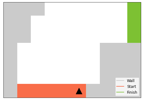
Let’s consider a ASCII representation of the map (or track) like this:
Here, S denotes a starting positiona, F denotes a finishing position, # denotes a wall, and denotes a road. We have this track as a 2D NumPy Array, and encode agent’s position as an index of this array.
Code
import numpy as npdef ascii_to_array(ascii_track: str) -> np.ndarray:"""Convert the ascii (string) map to a NumPy array.""" lines = [line for line in ascii_track.split("\n") iflen(line) >0] byte_lines = [list(bytes(line, encoding="utf-8")) for line in lines]return np.array(byte_lines, dtype=np.uint8)track = ascii_to_array(SMALL_TRACK)print(track)position = np.array([0, 0])track[tuple(position)] ==int.from_bytes(b'#', "big")
Then, agent’s velocity and acceleration are also naturally represented by an array. And, we represent an action as an index of an array consisting of all possible acceleration vetors:
The next step is to represent a transition function as a black box simulator. Note that we will visit another representation by transition matrix, but implementing the simulator is easier. Basically, the simulator should take an agent’s action and current state, and then return the next state. Let’s call this function step. However, let’s make it return some other things to make the implementation easier. Reward function sounds fairly easy to implement given the agent’s position. > The rewards are −1 for each step until the car crosses the finish line.
Also, we have to handle the termination of the episode. > Each episode begins in one of the randomly selected start states with both velocity components zero and ends when the car crosses the finish line.
So the resulting step function should return a tuple (state, reward, termination). The below cell contains my implementation of the simulator with matplotlib visualization. The step function is so complicated to handle the case where the agent goes through a wall, so readers are encouraged to just run their eyes through.
Code
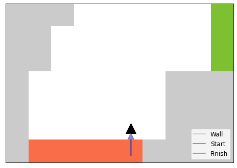
# collapse-hidefrom typing import List, NamedTuple, Optional, Tuplefrom IPython.display import displayfrom matplotlib import pyplot as pltfrom matplotlib.axes import Axesfrom matplotlib.colors import ListedColormapclass State(NamedTuple): position: np.ndarray velocity: np.ndarrayclass RacetrackEnv:"""Racetrack environment""" EMPTY =int.from_bytes(b" ", "big") WALL =int.from_bytes(b"#", "big") START =int.from_bytes(b"S", "big") FINISH =int.from_bytes(b"F", "big")def__init__(self, ascii_track: str, noise_prob: float=0.1, seed: int=0, ) ->None:self._track = ascii_to_array(ascii_track)self._max_height, self._max_width =self._track.shapeself._noise_prob = noise_probself._actions = np.array(list(itertools.product([-1, 0, 1], [-1, 0, 1])))self._no_accel =4self._random_state = np.random.RandomState(seed=seed)self._start_positions = np.argwhere(self._track ==self.START)self._state_indices =Noneself._ax =Noneself._agent_fig =Noneself._arrow_fig =Nonedef state_index(self, state: State) ->int:"""Returns a state index""" (y, x), (vy, vx) = statereturn y *self._max_width *25+ x *25+ vy *5+ vxdef _all_passed_positions(self, start: np.ndarray, velocity: np.ndarray, ) -> Tuple[List[np.ndarray], bool]:""" List all positions that the agent passes over. Here we assume that the y-directional velocity is already flipped by -1. """ maxv = np.max(np.abs(velocity))if maxv ==0:return [start], False one_step_vector = velocity / maxv pos = start +0.0 traj = []for i inrange(maxv): pos = pos + one_step_vector ceiled = np.ceil(pos).astype(int)ifself._is_out(ceiled):return traj, True traj.append(ceiled)# To prevent numerical issue traj[-1] = start + velocityreturn traj, Falsedef _is_out(self, position: np.ndarray) ->bool:"""Returns whether the given position is out of the map.""" y, x = positionreturn y <0or x >=self._max_widthdef step(self, state: State, action: int) -> Tuple[State, float, bool]:""" Taking the current state and an agents' action, returns the next state, reward and a boolean flag that indicates that the current episode terminates. """ position, velocity = stateifself._random_state.rand() <self._noise_prob: accel =self._actions[self._no_accel]else: accel =self._actions[action]# velocity is clipped so that only ↑→ directions are possible next_velocity = np.clip(velocity + accel, a_min=0, a_max=4)# If both of velocity is 0, cancel the accelerationif np.sum(next_velocity) ==0: next_velocity = velocity# List up trajectory. y_velocity is flipped to adjust the coordinate system. traj, went_out =self._all_passed_positions( position, next_velocity * np.array([-1, 1]), ) passed_wall, passed_finish =False, Falsefor track inmap(lambda pos: self._track[tuple(pos)], traj): passed_wall |= track ==self.WALL passed_finish |= track ==self.FINISHifnot passed_wall and passed_finish: # Goal!return State(traj[-1], next_velocity), 0, Trueelif passed_wall or went_out: # Crasshed to the wall or run outsidereturnself.reset(), -1.0, Falseelse:return State(traj[-1], next_velocity), -1, Falsedef reset(self) -> State:"""Randomly assigns a start position of the agent.""" n_starts =len(self._start_positions) initial_pos_idx =self._random_state.choice(n_starts) initial_pos =self._start_positions[initial_pos_idx] initial_velocity = np.array([0, 0])return State(initial_pos, initial_velocity)def render(self, state: Optional[State] =None, movie: bool=False, ax: Optional[Axes] =None, ) -> Axes:"""Render the map and (optinally) the agents' position and velocity."""ifself._ax isNoneor ax isnotNone:if ax isNone: _, ax = plt.subplots(1, 1, figsize=(8, 8)) ax.set_aspect("equal") ax.set_xticks([]) ax.set_yticks([])# Map the track to one of [0, 1, 2, 3] to that simple colormap works map_array = np.zeros_like(track) symbols = [self.EMPTY, self.WALL, self.START, self.FINISH]for i inrange(track.shape[0]):for j inrange(track.shape[1]): map_array[i, j] = symbols.index(self._track[i, j]) cm = ListedColormap( ["w", ".75", "xkcd:reddish orange", "xkcd:kermit green"] ) map_img = ax.imshow( map_array, cmap=cm, vmin=0, vmax=4, alpha=0.8, )if ax.get_legend() isNone: descriptions = ["Empty", "Wall", "Start", "Finish"]for i inrange(1, 4):if np.any(map_array == i): ax.plot([0.0], [0.0], color=cm(i), label=descriptions[i]) ax.legend(fontsize=12, loc="lower right")self._ax = axif state isnotNone:ifnot movie andself._agent_fig isnotNone:self._agent_fig.remove()ifnot movie andself._arrow_fig isnotNone:self._arrow_fig.remove() pos, vel = stateself._agent_fig =self._ax.plot(pos[1], pos[0], "k^", markersize=20)[0]# Show velocityself._arrow_fig =self._ax.annotate("", xy=(pos[1], pos[0] +0.2), xycoords="data", xytext=(pos[1] - vel[1], pos[0] + vel[0] +0.2), textcoords="data", arrowprops={"color": "xkcd:blueberry", "alpha": 0.6, "width": 2}, )returnself._axsmalltrack = RacetrackEnv(SMALL_TRACK)state = smalltrack.reset()print(state)display(smalltrack.render(state=state).get_figure())next_state, reward, termination = smalltrack.step(state, 7)print(next_state)smalltrack.render(state=next_state)
Note that the vertical velocity is negative, so that we can simply represent the coordinate by an array index.
Solve a small problem by dynamic programming
OK, now we have a simulator, so let’s solve the problem! However, before stepping into reinforcement learning, it’s better to compute an optimal policy in a small problem for sanity check. To do so, we need a transition matrix p, which is a \(|\mathcal{S}| \times |\mathcal{A}| \times |\mathcal{S}|\) NumPy array where p[i][j][k] is the probability of transiting from i to k when action j is taken. Also, we need a \(|\mathcal{S}| \times |\mathcal{A}| \times |\mathcal{S}|\) reward matrix r. Note that this representation is not general as \(R_t\) can be stochastic, but since the only stochasticity of rewards is the noise to actions in this problem, this notion suffices. It is often not very straightforward to get p and r from the problem definition, but basically we need to give 0-indexd indices to each state (0, 1, 2, ...) and fill the array. Here, I index each state by \(\textrm{Idx(S)} = y \times 25 \times W + x \times 25 + vy \times 5 + vx\), where \((x, y)\) is a position, \((vx, vy\)) is a velocity, and \(W\) is the width of the map.
Code
# collapse-hidefrom typing import Iterabledef get_p_and_r(env: RacetrackEnv) -> Tuple[np.ndarray, np.ndarray]:"""Taking RacetrackEnv, returns the transition probability p and reward fucntion r of the env.""" n_states = env._max_height * env._max_width *25 n_actions =len(env._actions) p = np.zeros((n_states, n_actions, n_states)) r = np.ones((n_states, n_actions, n_states)) *-1 noise = env._noise_probdef state_prob(*indices):"""Returns a |S| length zero-initialized array where specified elements are filled""" prob =1.0/len(indices) res = np.zeros(n_states)for idx in indices: res[idx] = probreturn res# List up all states and memonize starting states states = [] starting_states = []for y inrange(env._max_height):for x inrange(env._max_width): track = env._track[y][x]for y_velocity inrange(5):for x_velocity inrange(5): state = State(np.array([y, x]), np.array([y_velocity, x_velocity])) states.append(state)if track == env.START: starting_states.append(env.state_index(state))for state in states: position, velocity = state i = env.state_index(state) track = env._track[tuple(position)]# At a terminating state or unreachable, the agent cannot moveif ( track == env.FINISHor track == env.WALLor (np.sum(velocity) ==0and track != env.START) ): r[i] =0 p[i, :] = state_prob(i)# Start or empty stateselse:# First, compute next state probs without noise next_state_prob = []for j, action inenumerate(env._actions): next_velocity = np.clip(velocity + action, a_min=0, a_max=4)if np.sum(next_velocity) ==0: next_velocity = velocity traj, went_out = env._all_passed_positions( position, next_velocity * np.array([-1, 1]), ) passed_wall, passed_finish =False, Falsefor track inmap(lambda pos: env._track[tuple(pos)], traj): passed_wall |= track == env.WALL passed_finish |= track == env.FINISHif passed_wall or (went_out andnot passed_finish):# Run outside or crasheed to the wall next_state_prob.append(state_prob(*starting_states))else: next_state_idx = env.state_index(State(traj[-1], next_velocity)) next_state_prob.append(state_prob(next_state_idx))if passed_finish: r[i, j, next_state_idx] =0.0# Then linearly mix the transition probs with noisefor j inrange(n_actions): p[i][j] = ( noise * next_state_prob[env._no_accel]+ (1.0- noise) * next_state_prob[j] )return p, r
Then, let’s compute the optimal Q value by value iteration. So far, we only learned dynamic programming with discount factor \(\gamma\), so let’s use \(\gamma =0.95\) that is sufficiently large for this small problem. \(\epsilon = 0.000001\) is used as a convergence threshold. Let’s show the elapsed time and the required number of iteration.
It took longer that a second on my laptop, even for this small problem. Some technical notes on value iteration (\(R_\textrm{max} = 1.0\) is assumed for simplicity): - Each iteration takes \(O(|\mathcal{S}| ^ 2 |\mathcal{A}|)\) time - The required iteration number is bounded by \(\frac{\log \epsilon}{\gamma - 1}\) - In our case, \(\frac{\log \epsilon}{\gamma - 1} \approx 270\), so our computation converged quicker than theory - Thus the total computation time is bounded by \(O(|\mathcal{S}| ^ 2 |\mathcal{A}|\frac{\log \epsilon}{\gamma - 1})\) - For a convergence threshold \(\epsilon\), \(\max |V(s) - V^*(s)| < \frac{\gamma\epsilon}{1 - \gamma}\) is guranteed - In our case, \(\frac{\gamma\epsilon}{1 - \gamma} \approx 0.00002\) - This is called relative error
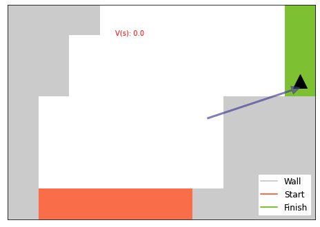
Let’s visualize the V value and an optimal trajectory. celluloid) is used for making an animation.
The computed optimal policy and value seems correct.
Monte-Carlo prediction
Then let’s try ‘reinforcement learning’. First, I implemeted ‘First visit Monte-Carlo prediction’, which evaluates a (Markovian) policy \(\pi\) by doing a simulation multiple times, and calculates the average of received returns. Here, I evaluate the optimal policy \(\pi^*\) obtained by value iteration.
Code
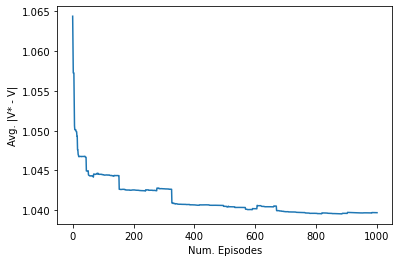
# collapse-hidefrom typing import Uniondef first_visit_mc_prediction( policy: Policy, env: RacetrackEnv, n_episodes: int, discount: float=0.95, record_all_values: bool=False,) -> Tuple[np.ndarray, List[np.ndarray]]:"""Predict value function corresponding to the policy by First-visit MC prediction""" n_states = env._max_width * env._max_height *25 v = np.zeros(n_states) all_values = []# Note that we have to have a list of returns for each state!# So the maximum memory usage would be Num.States x Num.Episodes all_returns = [[] for _ inrange(n_states)]for i inrange(n_episodes):if record_all_values: all_values.append(v.copy()) state = env.reset() visited_states = [env.state_index(state)] received_rewards = []# Rollout the policy until the episode endswhileTrue:# Sample an action from the policy action = policy(env.state_index(state))# Step the simulator state, reward, termination = env.step(state, action) visited_states.append(env.state_index(state)) received_rewards.append(reward)if termination:break# Compute return traj_len =len(received_rewards) returns = np.zeros(traj_len)# Gt = Rt when t = T returns[-1] = received_rewards[-1]# Iterating from T - 2, T - 1, ..., to 0for t inreversed(range(traj_len -1)):# Gt = Rt + γGt+1 returns[t] = received_rewards[t] + discount * returns[t +1] updated =set()# Update the valuefor i, state inenumerate(visited_states[: -1]):# If the state is already visited, skip itif state in updated:continue updated.add(state) all_returns[state].append(returns[i].item())# V(St) ← average(Returns(St)) v[state] = np.mean(all_returns[state])return v, all_valuesv, all_values = first_visit_mc_prediction( smalltrack_optimal_policy, smalltrack,1000, record_all_values=True,)value_diff = []for i, mc_value inenumerate(all_values + [v]): value_diff.append(np.mean(np.abs(mc_value - vi_result.v)))plt.plot(value_diff)plt.xlabel("Num. Episodes")plt.ylabel("Avg. |V* - V|")
Text(0, 0.5, 'Avg. |V* - V|')
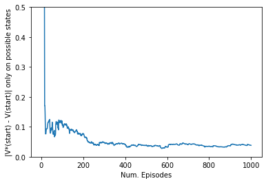
It looks like that the difference between \(V^*\) and the value function estimated by MC prediction converges after 600 steps, but it’s still larger than \(0\), because \(\pi^*\) doesn’t visit all states. Let’s plot the difference between value functions only on starting states.
Code
start_states = []for x inrange(1, 6): idx = smalltrack.state_index(State(position=np.array([6, x]), velocity=np.array([0, 0]))) start_states.append(idx)start_values = []for i, mc_value inenumerate(all_values + [v]): start_values.append(np.mean(np.abs(mc_value - vi_result.v)[start_states]))plt.plot(start_values)plt.xlabel("Num. Episodes")plt.ylabel("|V*(start) - V(start)| only on possible states")plt.ylim((0.0, 0.5))
Here, we can confirm that the estimated value certainly converged close to 0.0, while fractuating a bit. Note that the magnitude of fractuation is larger than the relative error we allowed for value iteration (\(0.00002\)), implying the difficulty of convergence.
Monte-Carlo Control
Now we successfully estimate \(V^\pi\) using Monte Carlo method, so then let’s try to learn a sub-optimal \(\pi\) directly using Monte Carlo method. In the textbook, three methods are introduced: - Monte Carlo ES (Exploring Starts) - On-policy first visit Monte Carlo Control - Off-policy first visit Monte Carlo Control
Here, let’s try all three methods and compare the resulting value functions. However, we cannot naively implement the pseudo code in the textbook, due to a ‘loop’ problem. Since the car that crashed into the wall is returned to a starting point, the episode length can be infinitte depending on a policy. As a remedy for this problem, I limit the length of the episode as \(H\). Supposing that we ignore the future rewards smaller than \(\epsilon\), how to set \(H\)? Just by solving \(\gamma^H R < \epsilon\), we get \(H > \frac{\log \epsilon}{\log \gamma}\), which is about \(270\) in case \(\gamma = 0.95\) and \(\epsilon = 0.000001\).
Below are the implementation of three methods. A few notes about implementation: - Monte Carlo ES requires a set of all possible states, which is implemented in valid_states function. - For On-Policy MC, \(\epsilon\) is decreased from 0.5 to 0.01 - We can use arbitary policy in Off-Policy MC, but I used the same \(\epsilon\)-soft policy as On-Policy MC.
Code
# collapse-hidedef valid_states(env: RacetrackEnv) -> List[State]: states = []for y inrange(env._max_height):for x inrange(env._max_width): track = env._track[y][x]if track == env.WALL:continuefor y_velocity inrange(5):for x_velocity inrange(5): state = State(np.array([y, x]), np.array([y_velocity, x_velocity]))if track != env.START and (x_velocity >0or y_velocity >0): states.append(state)return statesdef mc_es( env: RacetrackEnv, n_episodes: int, discount: float=0.95, record_all_values: bool=False, seed: int=999,) -> Tuple[np.ndarray, List[np.ndarray]]:"""Monte-Carlo Control with Exploring Starts""" n_states = env._max_width * env._max_height *25 n_actions =len(env._actions) random_state = np.random.RandomState(seed=seed) q = np.zeros((n_states, n_actions)) pi = random_state.randint(9, size=n_states) all_values = [] all_returns = [[[] for _ inrange(n_actions)] for _ inrange(n_states)] possible_starts = valid_states(env) max_episode_length =int(np.ceil(np.log(1e-6) / np.log(discount)))for i inrange(n_episodes):if record_all_values: all_values.append(q.copy()) state = possible_starts[random_state.choice(len(possible_starts))] visited_states = [env.state_index(state)] taken_actions = [] received_rewards = [] initial =Truefor _ inrange(max_episode_length):if initial:# Randomly sample the first action action = random_state.randint(9) initial =Falseelse:# Take an action following the policy action = pi[env.state_index(state)] taken_actions.append(action)# Step the simulator state, reward, termination = env.step(state, action) visited_states.append(env.state_index(state)) received_rewards.append(reward)if termination:break# Compute return traj_len =len(received_rewards) returns = np.zeros(traj_len)# Gt = Rt when t = T returns[-1] = received_rewards[-1]# Iterating from T - 2, T - 1, ..., to 0for t inreversed(range(traj_len -1)):# Gt = Rt + γGt+1 returns[t] = received_rewards[t] + discount * returns[t +1] updated =set()# Update the valuefor i, (state, action) inenumerate(zip(visited_states[:-1], taken_actions)):# If the state is already visited, skip itif (state, action) in updated:continue updated.add((state, action)) all_returns[state][action].append(returns[i].item())# Q(St, At) ← average(Returns(St, At)) q[state, action] = np.mean(all_returns[state][action]) pi[state] = np.argmax(q[state])return q, all_valuesdef on_policy_fist_visit_mc( env: RacetrackEnv, n_episodes: int, discount: float=0.95, epsilon: float=0.1, epsilon_final: float=0.1, record_all_values: bool=False, seed: int=999,) -> Tuple[np.ndarray, List[np.ndarray]]:"""On-policy first visit Monte-Carlo""" n_states = env._max_width * env._max_height *25 n_actions =len(env._actions) random_state = np.random.RandomState(seed=seed) q = np.zeros((n_states, n_actions)) pi = random_state.randint(9, size=n_states) all_values = [] all_returns = [[[] for _ inrange(n_actions)] for _ inrange(n_states)] possible_starts = valid_states(env) max_episode_length =int(np.ceil(np.log(1e-6) / np.log(discount))) epsilon_decay = (epsilon - epsilon_final) / n_episodesfor i inrange(n_episodes):if record_all_values: all_values.append(q.copy()) state = env.reset() visited_states = [env.state_index(state)] taken_actions = [] received_rewards = []for _ inrange(max_episode_length):# ε-soft policyif random_state.rand() < epsilon: action = random_state.randint(9)else: action = pi[env.state_index(state)] taken_actions.append(action)# Step the simulator state, reward, termination = env.step(state, action) visited_states.append(env.state_index(state)) received_rewards.append(reward)if termination:break# Below code is the same as mc_es# Compute return traj_len =len(received_rewards) returns = np.zeros(traj_len)# Gt = Rt when t = T returns[-1] = received_rewards[-1]# Iterating from T - 2, T - 1, ..., to 0for t inreversed(range(traj_len -1)):# Gt = Rt + γGt+1 returns[t] = received_rewards[t] + discount * returns[t +1] updated =set()# Update the valuefor i, (state, action) inenumerate(zip(visited_states[:-1], taken_actions)):# If the state is already visited, skip itif (state, action) in updated:continue updated.add((state, action)) all_returns[state][action].append(returns[i].item())# Q(St, At) ← average(Returns(St, At)) q[state, action] = np.mean(all_returns[state][action]) pi[state] = np.argmax(q[state]) epsilon -= epsilon_decayreturn q, all_valuesdef off_policy_mc( env: RacetrackEnv, n_episodes: int, discount: float=0.95, record_all_values: bool=False, epsilon: float=0.1, epsilon_final: float=0.1, seed: int=999,) -> Tuple[np.ndarray, List[np.ndarray]]:"""Off-policy MC control""" n_states = env._max_width * env._max_height *25 n_actions =len(env._actions) random_state = np.random.RandomState(seed=seed) q = np.zeros((n_states, n_actions)) c = np.zeros_like(q) pi = np.argmax(q, axis=1) all_values = [] possible_starts = valid_states(env) max_episode_length =int(np.ceil(np.log(1e-6) / np.log(discount))) epsilon_decay = (epsilon - epsilon_final) / n_episodesfor i inrange(n_episodes):if record_all_values: all_values.append(q.copy()) state = env.reset() visited_states = [env.state_index(state)] taken_actions = [] received_rewards = [] acted_optimally = []for _ inrange(max_episode_length):# ε-soft policyif random_state.rand() < epsilon: action = random_state.randint(9)else: action = pi[env.state_index(state)] acted_optimally.append(action == pi[env.state_index(state)]) taken_actions.append(action)# Step the simulator state, reward, termination = env.step(state, action) visited_states.append(env.state_index(state)) received_rewards.append(reward)if termination:break g =0 w =1.0for i, (state, action) inenumerate(zip(visited_states[:-1], taken_actions)): g = discount * g + received_rewards[i] c[state, action] += w q[state, action] += w / c[state, action] * (g - q[state, action]) pi[state] = np.argmax(q[state])if action == pi[state]:breakelse:if acted_optimally[i]: w *=1.0- epsilon + epsilon / n_actionselse: w *= epsilon / n_actions epsilon -= epsilon_decayreturn q, all_valuesmces_result = mc_es(smalltrack, 3000, record_all_values=True)on_mc_result = on_policy_fist_visit_mc( smalltrack,3000, epsilon=0.5, epsilon_final=0.01, record_all_values=True,)off_mc_result = off_policy_mc( smalltrack,3000, epsilon=0.5, epsilon_final=0.01, record_all_values=True,)
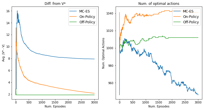
Let’s plot the results. Here I plotted the difference from the optimal value function and the number of states that the policy choices the optimal action.
Some observations from the results: - On-Policy MC converges to the optimal policy the fastest, though the convergence of its value function is the slowest - MC-ES struggles to distinguish optimal and non-optimal actions at some states, probably because of the lack of exploration during an episode. - Compared to MC-ES and On-Policy MC, the peak of value differences of Off-Policy MC is much milder. - A randomly initialized policy is often caught in a loop and cannot reach to the goal. The value of such a policy is really small (\(-1 -1 * 0.95 - 1 * 0.95^2 - ... \approx -20\)). However, Off-Policy MC uses important sampling to decay the rewards by uncertain actions, resulting the smaller value differences.
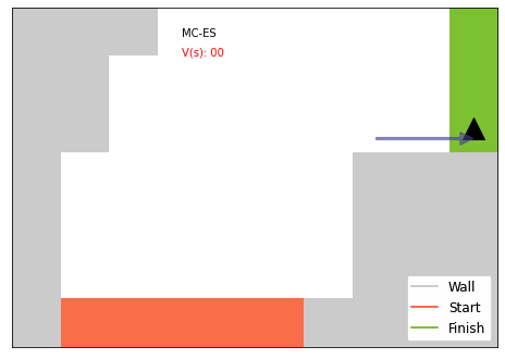
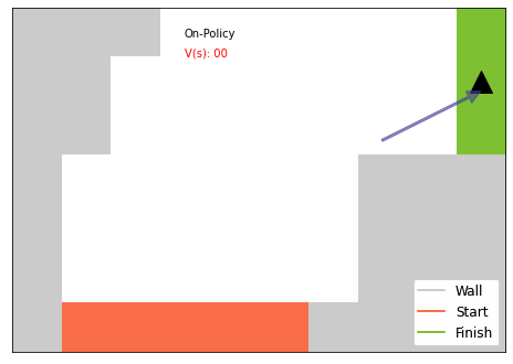
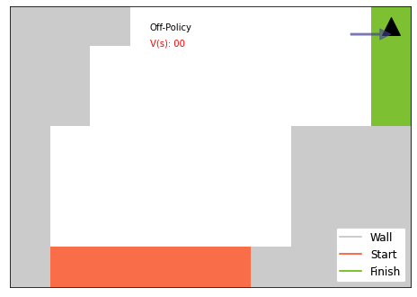
Here I visualized sampled plays from all three methods. On-Policy MC looks the most efficient.
Code
for q, name inzip([mces_result[0], on_mc_result[0], off_mc_result[0]], ["MC-ES", "On-Policy", "Off-Policy"]): display(show_rollout(smalltrack, lambda i: np.argmax(q[i]), np.argmax(q, axis=-1), name))